Pushing around 3D points $$[x, y, z]^T$$ is fundamentally different from 2D coordinates $$[x, y]^T$$ because suddenly, you have a flexible rotation axis (in 2D it is always the one coming out of the screen at $$[0, 0]^T$$. In case you are wondering, the $$^T$$ notation for "transpose" is just for nicer reading). Translation stays the same though. In the following, we will push one point around but ignore relating two or more points.
Given a point $$\vec{p} \in \R^3$$, we might think it exists in "the coordinate system" (CS), but more formally it has an origin $$\vec{o} = [0, 0, 0]^T$$ and three axes $$\vec{x} = [1, 0, 0]^T$$, $$\vec{y} = [0, 1, 0]^T$$, and $$\vec{z} = [0, 0, 1]^T$$, so in some sense $$\vec{p} = [p_x, p_y, p_z]^T$$ can be interpreted as $$\vec{o} + p_x \cdot \vec{x} + p_y \cdot \vec{y} + p_z \cdot \vec{z}$$, or in prose "start at $$\vec{o}$$, go $$p_x$$ along $$\vec{x}$$, then $$p_y$$ along $$\vec{y}$$, and finally $$p_z$$ along $$\vec{z}$$". The three axes (without $$\vec{o}$$) are called basis vectors because with them, we can reach any point in our space.
You probably already guessed why this might be relevant: We can have different axes and thus different bases. And we can have a different origin too; together these four form a new coordinate system ("space").
Easier to understand than rotation. You simply move $$\vec{p}$$ by adding a translation vector $$\vec{t} = [t_x, t_y, t_z]^T$$. Since matrix operations can combine rotation and translation, developers usually define the point as homogeneous coordinate $$\vec{p} = [x, y, z, 1]^T$$ and multiply it with a $$4 \times 4$$ translation matrix $$T = [ I^4 | \vec{t}] = \begin{bmatrix} 1 & 0 & 0 & t_x\\ 0 & 1 & 0 & t_y\\ 0 & 0 & 1 & t_z\\ 0 & 0 & 0 & 1 \end{bmatrix}$$, and then use the shifted point $$\vec{q} = T\cdot\vec{p} = \begin{bmatrix} 1 & 0 & 0 & t_x\\ 0 & 1 & 0 & t_y\\ 0 & 0 & 1 & t_z\\ 0 & 0 & 0 & 1 \end{bmatrix} \begin{bmatrix}p_x\\ p_y\\ p_z\\ 1 \end{bmatrix} = \begin{bmatrix} 1 p_x + 0 p_y + 0 p_z + t_x 1\\ 0 p_x + 1 p_y + 0 p_z + t_y 1\\ 0 p_x + 0 p_y + 1 p_z + t_z 1\\ 0 p_x + 0 p_y + 0 p_z + 1 \cdot 1 \end{bmatrix} = \begin{bmatrix} p_x + t_x\\ p_y + t_y\\ p_z + t_z\\ 1 \cdot 1 \end{bmatrix}$$, while ignoring its homogeneous $$1$$.
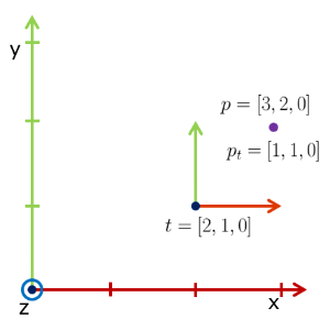
But what does that mean in terms of coordinate systems? Consider the image below.
We have a (larger) global coordinate system (GCS) $$B = I^4$$ with standard basis and origin $$\vec{0}$$, and a (smaller) local coordinate system (LCS) $$T = \begin{bmatrix} 1 & 0 & 0 & 2\\ 0 & 1 & 0 & 1\\ 0 & 0 & 1 & 0\\ 0 & 0 & 0 & 1 \end{bmatrix}$$ with standard basis but origin $$\vec{t} = [2, 1, 0]^T$$ (keeping the z-plane simple for the moment is a bit cheated, just so we can draw in 2D). Within the GCS a point $$\vec{p} = [3, 2, 0]^T$$ exists, and within the LCS the very same point would be $$\vec{p}_t = [1, 1, 0]^T$$.
A change of basis here means $$T$$ is interpreted as local2global transformation in the sense that $$T \cdot \vec{p}_t = \vec{p}$$ transforms any point from LCS to GCS, and the global2local $$T^{-1} = \begin{bmatrix} 1 & 0 & 0 & -2\\ 0 & 1 & 0 & -1\\ 0 & 0 & 1 & -0\\ 0 & 0 & 0 & 1 \end{bmatrix}$$ the other way around. Most obvious when applied to $$\vec{p}_t = \vec{0}$$ where the origin of $$T$$ is just $$\vec{t}$$ in the GCS.
A wondrous thing, we will always rotate around $$\vec{0}$$, no exceptions. If you want to rotate around another point $$\vec{r}$$, shift your $$\vec{p}$$ into that LCS first such that $$\vec{r}$$ becomes the new origin; that looks like $$ (R \cdot (\vec{p} - \vec{r})) + \vec{r}$$ or in prose "take $$\vec{p}$$, subtract $$\vec{r}$$ so that $$\vec{r}$$ is the new $$\vec{0}$$, apply rotation $$R$$, then shift result back to original coordinate system".
The second wondrous thing is that any rotation can be expressed with just one rotation axis. The most basic way of thinking is "rotation around the $$\vec{x}$$, $$\vec{y}$$ and $$\vec{z}$$ axis" with angles $$[r_x, r_y, r_z]$$, where the order is important and usually $$\vec{x} \rarr \vec{y} \rarr \vec{z}$$. Another way of thinking is the decidedly alien quaternions.
Our way: Think of a local coordinate system $$R$$ consisting of orthonormal vectors $$\vec{u}$$, $$\vec{v}$$ and $$\vec{w}$$ which are the LCS versions of $$\vec{x}$$, $$\vec{y}$$ and $$\vec{z}$$, in the sense that $$B = \begin{bmatrix} | & | & |\\ \vec{x} & \vec{y} & \vec{z}\\ | & | & | \end{bmatrix} = \begin{bmatrix} 1 & 0 & 0\\ 0 & 1 & 0\\ 0 & 0 & 1\end{bmatrix}$$ (GCS) and $$R = \begin{bmatrix} | & | & |\\ \vec{u} & \vec{v} & \vec{w}\\ | & | & | \end{bmatrix}$$ (LCS). A rotation is then $$\vec{q} = R \cdot \vec{p} = \begin{bmatrix} u_x & v_x & w_x\\ u_y & v_y & w_y\\ u_z & v_z & w_z \end{bmatrix} \begin{bmatrix} p_x\\ p_y\\ p_z\end{bmatrix} = \begin{bmatrix} u_x p_x + v_x p_y + w_x p_z\\ u_y p_x + v_y p_y + w_y p_z\\ u_z p_x + v_z p_y + w_z p_z\\ \end{bmatrix} = p_x \vec{u} + p_y \vec{v} + p_z \vec{w}$$ or in prose "go $$p_x$$ along $$\vec{u}$$, then $$p_y$$ along $$\vec{v}$$, and then finally $$p_z$$ along $$\vec{w}$$".
And in terms of changing coordinate systems? Again, consider the image below.
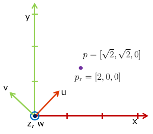
Rotated 45° counter-clockwise around the global z-axis, the local coordinate system is $$R = \begin{bmatrix} | & | & |\\ \vec{u} & \vec{v} & \vec{w}\\ | & | & | \end{bmatrix} = \begin{bmatrix} \sqrt{\frac{1}{2}} & -\sqrt{\frac{1}{2}} & 0\\ \sqrt{\frac{1}{2}} & \sqrt{\frac{1}{2}} & 0\\ 0 & 0 & 1 \end{bmatrix}$$ such that the global point $$\vec{p} = [\sqrt{2}, \sqrt{2}, 0]^T$$ is the same as the local point $$\vec{p}_r = [2, 0, 0]^T$$, in prose "2 along $$\vec{u}$$, 0 along $$\vec{v}$$, 0 along $$\vec{w}$$". Again, this means $$R$$ is local2global such that $$\vec{p} = R \cdot \vec{p}_r = \begin{bmatrix} \sqrt{\frac{1}{2}} & -\sqrt{\frac{1}{2}} & 0\\ \sqrt{\frac{1}{2}} & \sqrt{\frac{1}{2}} & 0\\ 0 & 0 & 1 \end{bmatrix} \begin{bmatrix} 2\\ 0\\ 0 \end{bmatrix} = \begin{bmatrix} \sqrt{\frac{1}{2}} \cdot 2\\ \sqrt{\frac{1}{2}} \cdot 2\\ 0 \end{bmatrix} = \begin{bmatrix} \sqrt{2}\\ \sqrt{2}\\ 0 \end{bmatrix}$$ and $$R^{-1} = R^T = \begin{bmatrix} \text{---} & \vec{u} & \text{---}\\ \text{---} & \vec{v} & \text{---}\\ \text{---} & \vec{w} & \text{---} \end{bmatrix} = \begin{bmatrix} \sqrt{\frac{1}{2}} & \sqrt{\frac{1}{2}} & 0\\ -\sqrt{\frac{1}{2}} & \sqrt{\frac{1}{2}} & 0\\ 0 & 0 & 1 \end{bmatrix}$$ is the global2local transform that reverts it (note: $$R^T = R^{-1}$$ is only true for orthogonal matrixes).
Now we combine rotation $$R$$ and translation $$T$$ to produce a full rigid transformation matrix $$S = [R | \vec{t}] = \begin{bmatrix} | & | & | & |\\ \vec{u} & \vec{v} & \vec{w} & \vec{t}\\ | & | & | & |\\ 0 & 0 & 0 & 1 \end{bmatrix} = \begin{bmatrix} r_{00} & r_{01} & r_{00} & t_x\\ r_{10} & r_{11} & r_{10} & t_y\\ r_{20} & r_{21} & r_{20} & t_z\\ 0 & 0 & 0 & 1 \end{bmatrix}$$ with again the last row being used for homogeneous coordinates. When applying that matrix on a point with $$\vec{q} = S \cdot \vec{p}$$, the rotation is performed first, then the translation second. So rotation is around $$\vec{0}$$ as usual, and the rotation-then-translation can be seen as $$S = T \cdot R = \begin{bmatrix} I^3 & \vec{t}\\ 0 & 1\end{bmatrix} \begin{bmatrix} R & 0\\ 0 & 1\end{bmatrix} = \begin{bmatrix} 1 & 0 & 0 & t_x\\ 0 & 1 & 0 & t_y\\ 0 & 0 & 1 & t_z\\ 0 & 0 & 0 & 1 \end{bmatrix} \begin{bmatrix} r_{00} & r_{01} & r_{00} & 0\\ r_{10} & r_{11} & r_{10} & 0\\ r_{20} & r_{21} & r_{20} & 0\\ 0 & 0 & 0 & 1 \end{bmatrix} = \begin{bmatrix} r_{00} & r_{01} & r_{00} & t_x\\ r_{10} & r_{11} & r_{10} & t_y\\ r_{20} & r_{21} & r_{20} & t_z\\ 0 & 0 & 0 & 1 \end{bmatrix}$$, same as before.
For coordinate systems, consider the image below.
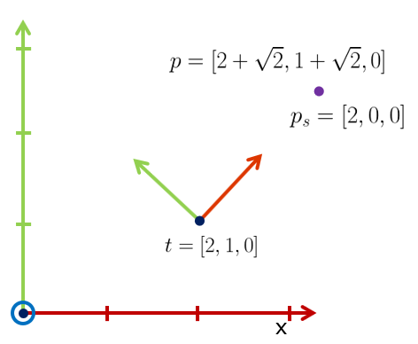
The (larger) GCS has standard basis and origin, and the (smaller) LCS combines the translation and rotation of the previous two images, with origin $$\vec{t} = [2, 1, 0]^T$$, rotation axes $$\vec{u} = [\sqrt{\frac{1}{2}}, \sqrt{\frac{1}{2}}, 0]^T$$, $$\vec{v} = [-\sqrt{\frac{1}{2}}, \sqrt{\frac{1}{2}}, 0]^T$$, $$\vec{w} = [0, 0, 1]^T$$. This leads to a local2global rigid transformation $$S = [R | \vec{t}] = \begin{bmatrix} \sqrt{\frac{1}{2}} & -\sqrt{\frac{1}{2}} & 0 & 2\\ \sqrt{\frac{1}{2}} & \sqrt{\frac{1}{2}} & 0 & 1\\ 0 & 0 & 1 & 0\\ 0 & 0 & 0 & 1 \end{bmatrix}$$ where a local point $$\vec{p}_s = [2, 0, 0]^T$$ (LCS) has a corresponding global point $$\vec{p} = S \cdot \vec{p}_s = \begin{bmatrix} \sqrt{\frac{1}{2}} & -\sqrt{\frac{1}{2}} & 0 & 2\\ \sqrt{\frac{1}{2}} & \sqrt{\frac{1}{2}} & 0 & 1\\ 0 & 0 & 1 & 0\\ 0 & 0 & 0 & 1 \end{bmatrix} \begin{bmatrix} 2\\ 0\\ 0\\ 1 \end{bmatrix} = \begin{bmatrix} \sqrt{\frac{1}{2}} \cdot 2 - \sqrt{\frac{1}{2}} \cdot 0 + 0 \cdot 0 + 2 \cdot 1\\ \sqrt{\frac{1}{2}} \cdot 2 + \sqrt{\frac{1}{2}} \cdot 0 + 0 \cdot 0 + 1 \cdot 1\\ 0 + 0 + 0 + 0\\ 0 + 0 + 0 + 1 \end{bmatrix} = \begin{bmatrix} 2 + \sqrt{2}\\ 1 + \sqrt{2}\\ 0\\ 1 \end{bmatrix} \approx \begin{bmatrix} 3.4\\ 2.4\\ 0 \end{bmatrix}$$ (GCS).
As for the reverse global2local transform, the inverse $$S^{-1}$$ would first need to back-translate, then do the back-rotation. Armed with the rule $$(A \cdot B)^{-1} = B^{-1} \cdot A^{-1}$$ from linear algebra, we can formulate the rotation-then-translation backwards as $$S^{-1} = (T \cdot R)^{-1} = R^{-1} \cdot T^{-1}$$, which confirms our back-translate-then-back-rotate assumption. And we know that the orthogonal $$R^{-1} = R^T$$, which gives us $$S^{-1} = R^T \cdot T^{-1}$$.
Numerically the inverse can be further simplified as $$S^{-1}= \left ( \begin{bmatrix} I & \vec{t}\\ 0 & 1\end{bmatrix} \begin{bmatrix} R & 0\\ 0 & 1\end{bmatrix} \right )^{-1} = \begin{bmatrix} R & 0\\ 0 & 1\end{bmatrix}^{-1} \begin{bmatrix} I & \vec{t}\\ 0 & 1\end{bmatrix}^{-1} = \begin{bmatrix} R^T & 0\\ 0 & 1\end{bmatrix} \begin{bmatrix} I & -\vec{t}\\ 0 & 1\end{bmatrix} = \begin{bmatrix} R^T & -R^T\vec{t}\\ 0 & 1\end{bmatrix}$$ with the intuition being that if you rotate a far-out point, you need to apply the rotation also to the LCS origin before going that far back.
And with that, we are through pushing a point around using linear 4x4 transformations. I hope you could get some nice intuition to complement your mathematical knowledge. Have a nice day!
EOF (Sep:2021)